[#4 Deep Dive] Fine-tuning your LLM efficiently with Hugging Face's 🤗 PEFT
Dive into the world of efficient fine-tuning with 🤗 PEFT.
⚡️ TL;DR for Time-Crunched BuildAIers:
You just got your hands on Llama 3.3 and are eager to fine-tune it on an internal dataset. But then you check the model card and realize it has 70,000,000,000 parameters. Yeah, that’s a 7 followed by 10 zeros! Fine-tuning all of them? That sounds like a nightmare.
Or does it?
Enter Parameter Efficient Fine Tuning (PEFT). With PEFT, you don’t have to adjust all 70 billion parameters. Instead, you can apply clever techniques like those outlined in research papers, such as LoRA, to achieve impressive results with minimal computational cost.
So, happy coding!
Or you could just use 🤗 PEFT.
Hugging Face’s PEFT library brings together the latest PEFT techniques, making fine-tuning large models easier. The library implements several PEFT techniques, such as:
✅ LoRA
✅ (IA)³
✅ P-tuning
✅ Prefix tuning
✅ Prompt tuning
In this article, we will explore the 🤗 PEFT library by focusing on two key implementations: LoRA and (IA)³. By the end, you will gain a deeper understanding of:
The fundamentals of fine-tuning Large Language Models (LLMs)
How PEFT enables efficient fine-tuning
The transformer architecture and how to choose the right modules for fine-tuning
LoRA: How it works and how to implement it using 🤗 PEFT
(IA)³: Its functionality, practical implementation with 🤗 PEFT, and what it stands for
Let's dive in. 🚀
A Quick Overview of Fine-Tuning Language Models
Fine-tuning Large Language Models (LLMs) is a technique for extending their capabilities to perform new tasks.
LLMs are typically pretrained on massive datasets, giving them broad language understanding.
However, they are not inherently specialized for specific tasks. To make them proficient in areas like question answering, summarization, and conversation, they require additional fine-tuning.
In the early days of fine-tuning, all of a model’s parameters were adjusted. The process was manageable when LLMs had only millions of parameters.
However, modern LLMs often contain billions of parameters, making full fine-tuning computationally expensive and impractical.
To solve this problem, researchers came up with Parameter Efficient Fine-Tuning (PEFT) techniques. These techniques make it possible to fine-tune models while reducing the amount of work that needs to be done and the money that needs to be spent.
📝 SIDE NOTE:
Weights and parameters are often used interchangeably, but there is a subtle distinction between them. Parameters can be thought of as variables in programming, while weights represent the actual values stored in them.
What is Parameter-Efficient Fine-Tuning (PEFT)?
PEFT is not a single technique but a family of methods designed to fine-tune LLMs efficiently by reducing the number of trainable parameters, making fine-tuning more computationally and memory efficient.
There are several PEFT techniques, with new ones continuously being developed, but they generally fall into three main categories:
Addition-based: Introduces trainable modules (adapters) into the model while keeping the original parameters frozen.
Selection-based: Fine-tunes specific modules of the model while keeping the rest frozen.
Reparameterization-based: It introduces trainable modules that serve as reparameterized versions of the original modules but with smaller dimensions.
There are several implementations of PEFT techniques, but most focus on only one specific method. If you are looking for a comprehensive solution that supports multiple PEFT techniques, you have two main options: 🤗 PEFT and Adapters.
This article will primarily focus on 🤗 PEFT, the Parameter Efficient Fine-Tuning library developed by the Hugging Face team.
🤗 PEFT: Hugging Face’s PEFT implementation
The PEFT library by Hugging Face seamlessly applies state-of-the-art PEFT techniques to AI models, allowing for fine-tuning LLMs and diffusion models. It also seamlessly integrates with other Hugging Face libraries, such as Transformers and Diffusers.
This article will focus on applying the 🤗 PEFT library to LLMs in the Transformers library.
A quick breakdown of 🤗 PEFT
The 🤗 PEFT API closely resembles that of the Transformers library and consists of two key components:
PEFT Configurations
PEFT Models
PEFT configurations define the settings for a specific PEFT technique, allowing it to be customized accordingly. In the 🤗 PEFT library, all configurations are subclasses of the PeftConfig class.
The PeftConfig class allows you to specify which PEFT technique is being used and the task type. The PEFT library supports six task types:
SEQ_CLS(Sequence Classification): Used for sentiment analysis and topic classification tasks.CAUSAL_LM(Causal Language Modeling): Used for autoregressive language modeling, where tokens are generated one token at a time (e.g., GPT-style models).SEQ_2_SEQ_LM(Sequence-to-Sequence Language Modeling): Used for machine translation and text summarization tasks.TOKEN_CLS(Token Classification): Used for tasks like Named Entity Recognition (NER) and Part-of-Speech (POS) tagging.QUESTION_ANS(Question Answering): Used for extractive question-answering tasks, where the model finds answers from a given context.FEATURE_EXTRACTION(Feature Extraction): Used when the model is needed for embedding generation rather than classification or generation.
Each PeftConfig subclass has its own set of configurations, which are equivalent to the hyperparameters of the corresponding PEFT technique. Another crucial parameter defined in the configuration is target_modules, which specifies the modules of the LLM that will be fine-tuned.
After creating a configuration, it can be applied to a transformer model, resulting in a PeftModel, a modified version of the original model with additional modules designed for efficient fine-tuning.
🤗 PEFT supports a range of Parameter-Efficient Fine-Tuning techniques, including prompt based methods like P-tuning, Prefix Tuning, and Prompt Tuning.
However, this article focuses on LoRA and (IA)³, representing reparameterization-based and addition-based approaches, respectively. Understanding these two techniques will provide a solid foundation for working with other methods in the 🤗 PEFT library.
A Quick Overview of the Transformer Architecture
When fine-tuning models with PEFT techniques, it is essential to understand the model's architecture to determine which modules to fine-tune. For LLMs, this means having a solid grasp of the transformer architecture, as it forms the foundation of most modern LLMs.
In this section, we will take a quick detour to explore the transformer architecture and identify the key components that play a crucial role in applying PEFT techniques effectively.
Like every deep learning model, the transformer consists of multiple layers that process data as vectors, applying transformations to extract meaningful representations. When it comes to PEFT, the two most essential components of the transformer are:
Linear Layers
Attention Mechanism
Linear Layer
In the transformer architecture, the linear layers are used in the feedforward networks and projection layers, where they use linear transformation to transform embeddings and intermediate representations. They play a crucial role in adjusting the dimensionality of data and refining learned features before passing them to the next stage of processing.
In the transformer architecture, linear layers are used in feedforward networks and projection layers to apply linear transformations to embeddings and intermediate representations. They are essential for adjusting dimensionality, refining learned features, and preparing data for the next processing stage.
Down Projections
Down projections are a type of linear layer that apply a linear transformation to reduce the dimensionality of an input vector using a weight matrix. This process compresses information while preserving key features.
For example, in the video above, an input vector with dimensions 1 × 4 is multiplied by a weight matrix of 4 × 3, resulting in an output vector of 1 × 3. This reduction in size qualifies as a down projection since the dimensionality of the vector decreases through the transformation.
Up Projections
Up projections are the opposite of down projections. They are linear layers that apply a linear transformation to increase the dimensionality of an input vector using a weight matrix. This expands the feature space, helping the model capture more complex representations.
For example, in the video above, a 1 × 3 input vector is multiplied by a 3 × 4 weight matrix, producing a 1 × 4 output vector. This increase in dimensionality makes it an up projection.
Attention Mechanism
The key breakthrough in the transformer architecture is the attention mechanism, specifically self-attention. This mechanism allows each input token to attend to all other tokens in the sequence, including itself. For example, in the sentence:
"The man wears a white tie."
The word "man" pays attention to every other word in the sequence, as well as itself. Each token evaluates the relevance of other tokens, determining which ones are most important to understanding its meaning.
To achieve this, the attention mechanism relies on the attention equation:
This equation involves three key matrices: Query (Q), Key (K), and Value (V). These matrices are derived by multiplying the input embeddings with their respective weight matrices WQ, WK, WV.
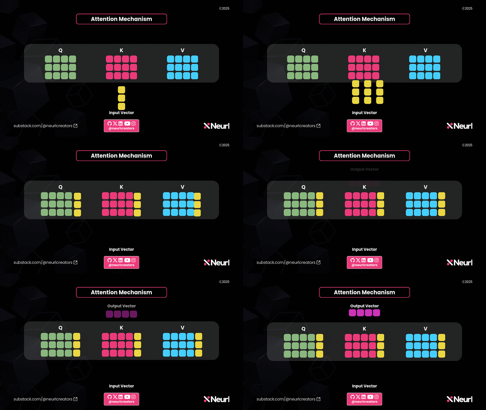
During training, the transformer updates these weight matrices, adjusting them to improve performance. This detail is crucial because when using Parameter Efficient Fine-Tuning (PEFT), we modify these weight matrices in a more efficient way.
LoRA: A Parameter-Efficient Fine-Tuning Technique
In 2021, researchers at Microsoft faced a significant challenge while working with GPT-3. The model had 175 billion parameters, making fine-tuning highly inefficient. They encountered the following issues:
Fine-tuning the entire model for downstream tasks was computationally expensive.
Adapting the model to new tasks required replacing all the weights, which was impractical.
Storing multiple fine-tuned versions of the model demanded enormous storage capacity.
To solve these problems, they introduced LoRA (Low-Rank Adaptation), a technique that enables efficient fine-tuning without modifying all the original weights.
LoRA uses reparameterization to fine-tune a large language model efficiently. Instead of directly fine-tuning the model's weights, LoRA introduces reparameterized weight matrices, which are then fine-tuned. Let’s dive deeper into how this works.
How LoRA Works
LoRA employs two key techniques that make it an effective PEFT method. The first technique is applied during fine-tuning, where LoRA introduces low-rank adapters to modify only a subset of the model’s weights.
The second technique comes into play during inference, where LoRA merges the fine-tuned adapters with the original model weights, ensuring there is no additional computational overhead. Let’s explore each of these techniques in detail.
Rank Decomposition: The Secret Sauce Behind LoRA
LoRA leverages rank decomposition to fine-tune its parameters. This concept originates from linear algebra, and the researchers behind LoRA found a clever way to apply it to fine-tuning language models.
Here's how rank decomposition works:
Given a matrix A
The matrix A has dimensions M × N.
Decomposing A into two smaller matrices
A is factorized into two matrices:
C with dimensions M × r
F with dimensions r × N
Understanding the rank (r)
r is the rank of the decomposition.
It is typically much smaller than M and N, reducing computational complexity.
Reconstructing the original matrix
When C and F are multiplied, they approximate the original M × N matrix.
This allows for a more efficient representation while retaining key information.
This rank decomposition technique is at the core of how LoRA optimizes fine-tuning in large models.
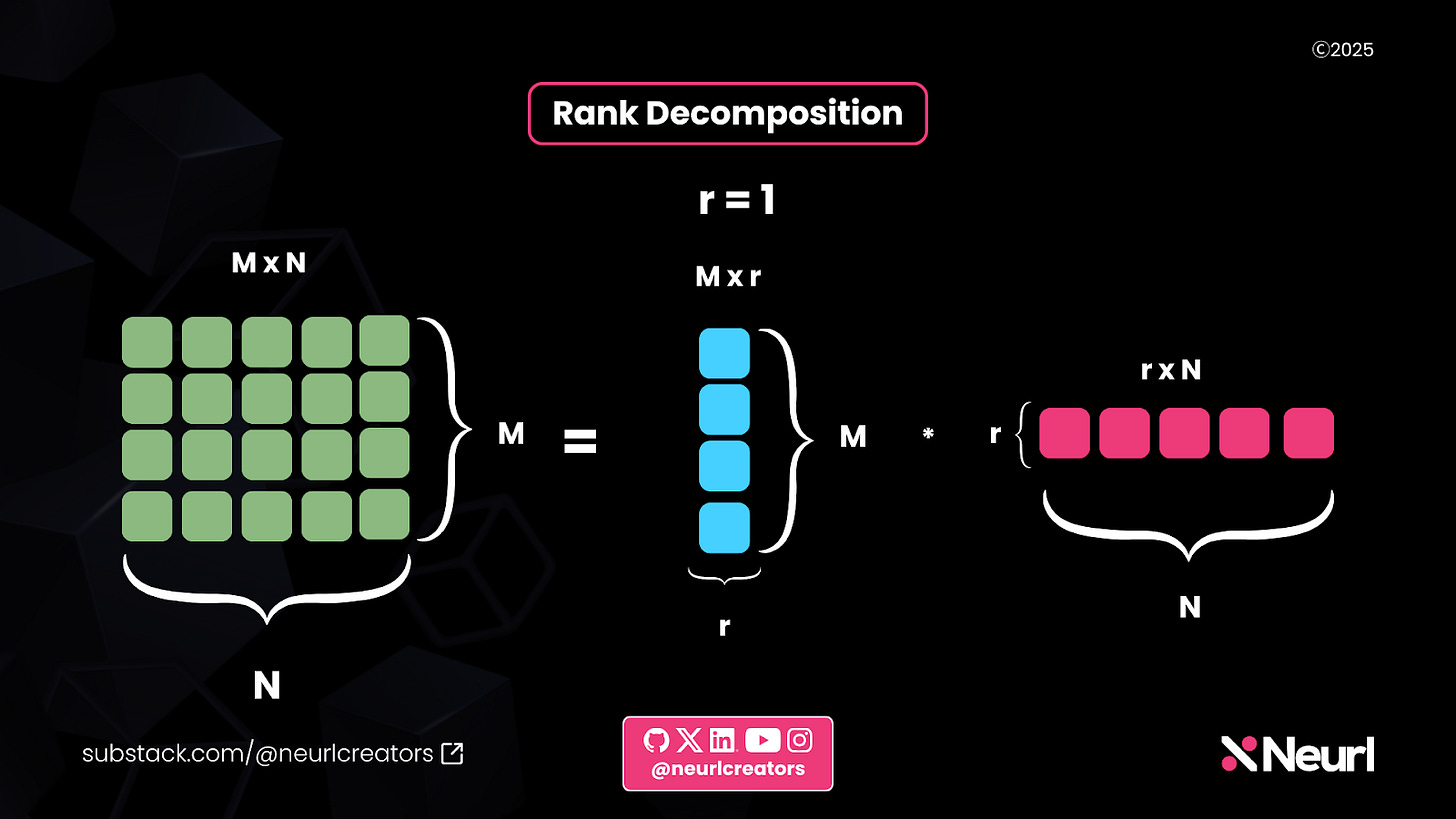
In the image above, we start with a green matrix of dimensions M × N. In this example:
M = 4 and N = 5, resulting in a 4 × 5 matrix with 20 elements.
However, this matrix can be decomposed into two smaller matrices, shown in blue and pink in the image. These matrices rank 1, meaning they provide a lower-dimensional representation of the original matrix.
The blue matrix has the same number of rows as the original green matrix (M = 4) and a single column, making its dimensions 4 × 1.
The pink matrix has the same number of columns as the original green matrix (N = 5) and a single row, making its dimensions 1 × 5.
By using this decomposition, we reduce the total number of elements to 4 + 5 = 9, which is significantly smaller than the original 20. This results in an 11× reduction in size. This reduced size in the number of elements in the decomposed matrix is the key to what makes LoRA efficient.
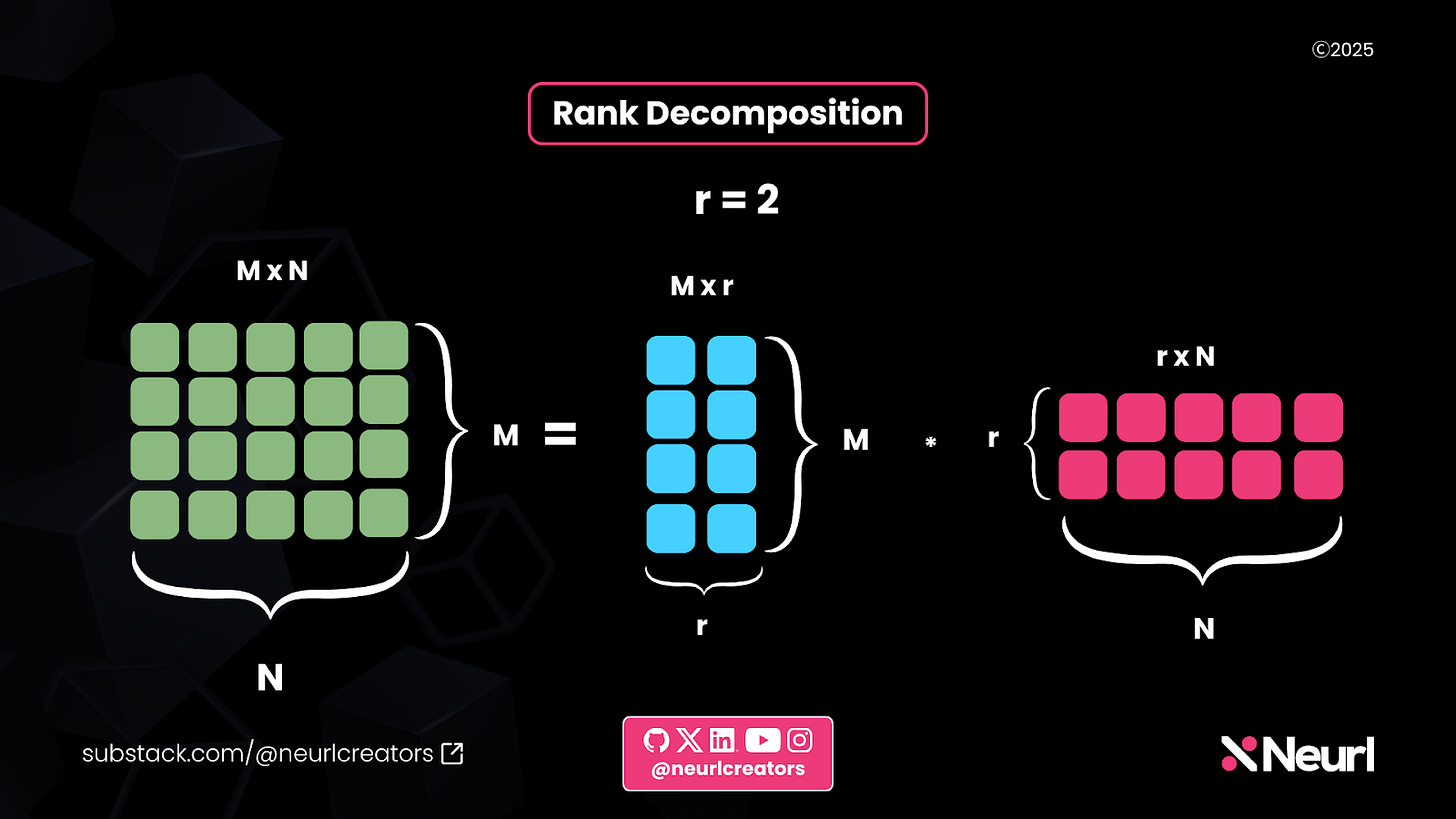
In this example, the rank is 2, meaning the decomposed matrices have slightly larger dimensions than in the previous case:
The blue matrix now has dimensions M × 2, which equals 4 × 2.
The pink matrix has dimensions 2 × N, which equals 2 × 5.
Although these matrices are larger than those in the first example, their total number of elements is 18, which is still 2 elements fewer than the original green matrix. This demonstrates how increasing the rank provides a better approximation while still reducing the overall parameter count.
Efficiently fine-tuning parameters using rank decomposition
We've seen the power of rank decomposition, but how does LoRA leverage it to fine-tune an LLM efficiently? Here’s how it works:
Freezing the LLM’s weights – LoRA keeps the original model weights frozen.
Decomposing the weight matrix dimensions – It takes the dimensions of a weight matrix from the LLM, whether from the linear layers or attention mechanism, and applies rank decomposition.
Fine-tuning only the decomposed matrices – Instead of training the full weight matrix, LoRA trains the smaller decomposed matrices, significantly reducing the number of trainable parameters.
Adapting the new weights to the frozen model
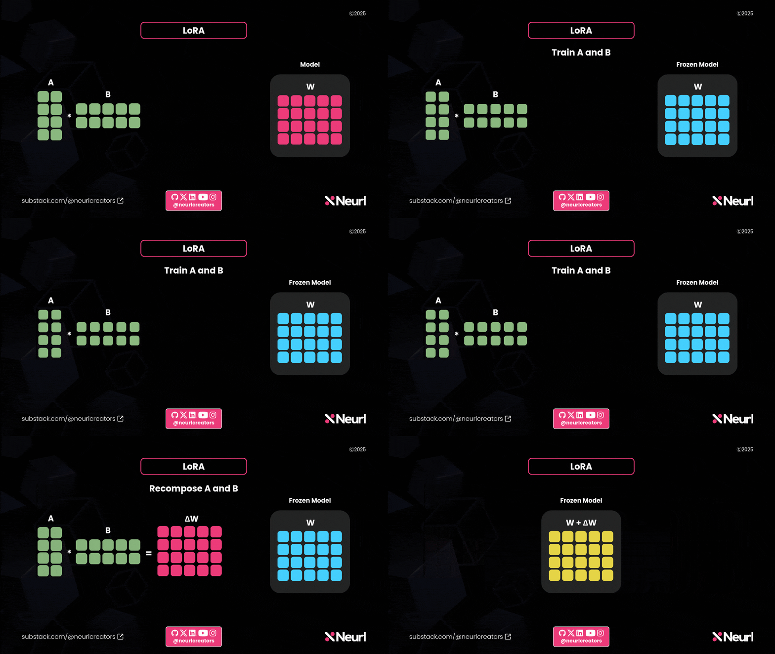
The next stage after rank decomposition is the adaptation stage. Despite its name, LoRA does not use adapters. Unlike traditional adapters, which introduce new weights to an LLM, LoRA takes a different approach. It recomposes the matrices from the decomposition stage and performs a simple addition between the trained decomposed weights and the original LLM weights. This process introduces no additional computational overhead, making LoRA an efficient fine-tuning method.
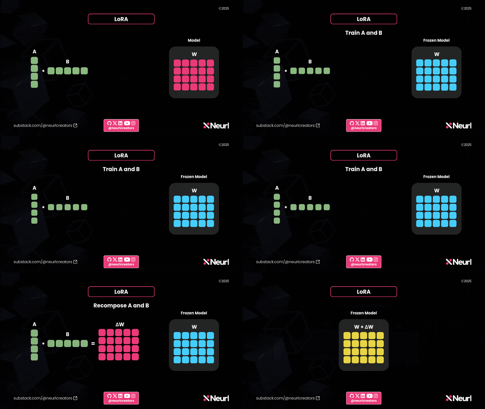
The video above demonstrates how LoRA works. Matrices A and B represent the trainable LoRA weights. After fine-tuning, these weights are composed into a matrix that matches the size of the original weight matrix in the frozen model. This newly formed matrix is then added to the model, enabling it to perform new tasks.
The video below shows an example of LoRA with rank 2. The original paper experimented with various ranks ranging from 1 to 64. The LoRA rank is a hyperparameter that can be adjusted to achieve optimal results.
Now that we have seen the LoRA theory, let’s see how we can use LoRA in the real world using 🤗 PEFT.
Using LoRA in 🤗 PEFT
To use LoRA, we first need to install the required libraries:
pip install peft transformers Once the installation is complete, the next step is to choose a model for fine-tuning. In this example, I will use Llama 3.2 1B, a relatively small model that can run on platforms like Google Colab with the right optimizations. However, you can choose any model that fits your needs.
Next, load the Llama model and tokenizer. After loading, we can inspect the model’s architecture.
From the image above, you can see the full architecture of the Llama 3.2 1B model. The two layers of particular interest are the self_attn and mlp layers. Now, let’s set up our LoRA model.
First, we import LoraConfig, which is used to configure LoRA, and get_peft_model, which applies the configuration to our Llama model.
In the configuration, we set r = 2, which defines the rank of the LoRA adaptation. We also specify the task type as CAUSAL_LM and use target_modules to determine which parts of the model LoRA should modify. To keep the output simple, I selected q_proj from the self_attn module and up_proj from the mlp module. With this setup, our LoRA module is ready. Let’s examine it.
If you look closely, you will notice that our model has changed. It is now a PEFTModel. More importantly, the q_proj and up_proj layers have additional modules. These modules are lora_A and lora_B. They have a rank of 2, as we specified in the configuration. This setup mirrors how our earlier diagrams depicted rank decomposition with a rank of 2.
When the PEFT model is fine-tuned, only these LoRA weights lora_A and lora_B are updated, while the main model weights remain frozen.
And that is it. This is how LoRA works in 🤗 PEFT. Now, you can use the Hugging Face Trainer class or the Trainer classes from TRL to fine-tune the model.
LoRA Variants in 🤗 PEFT
Several LoRA variants are in the 🤗 PEFT library, each leveraging some form of low-rank decomposition to achieve efficient parameter fine-tuning. Regardless of the variant, the process remains the same: Create a PeftConfig for the specific PEFT technique, then use it to initialize a PeftModel, which can be trained accordingly.
Here are some notable LoRA variants:
AdaLoRA: Adaptive LoRA dynamically allocates parameters to the most important modules, optimizing efficiency.
LoHA: Low-Rank Hadamard Product (LoHA) replaces standard matrix multiplication in LoRA with a Hadamard product.
LoKr: Low-Rank Kronecker Product (LoKr) takes a similar approach to LoHA but uses a Kronecker product instead.
X-LoRA: Mixture of LoRA Experts (X-LoRA) integrates LoRA with the mixture of experts approach for enhanced adaptability.
QLoRA: Combines LoRA with quantization (via bitsandbytes) to reduce memory usage while maintaining fine-tuning efficiency.
Want to explore LoRA variants in more detail? Dive into the 🤗 PEFT documentation on LoRA methods for a detailed exploration.
Infused Adapter by Inhibiting and Amplifying Inner Activations: A more efficient PEFT technique
The next PEFT technique we will explore is Infused Adapter by Inhibiting and Amplifying Inner Activations. Yes, that is a mouthful, so we will call it (IA)³. Before diving into how to use it with 🤗 PEFT, let's first understand its theory, how it differs from LoRA, and, most importantly, why it has such a unique name.
How (IA)³ Works and How it differs from LoRA
(IA)³ is an addition-based PEFT method. Unlike LoRA, which reparameterizes model weights for fine-tuning, (IA)³ does not modify existing parameters. Instead, it introduces additional parameters in the form of scaling vectors.
Despite this addition, (IA)³ is even more parameter-efficient than LoRA. LoRA adds low-rank weight matrices to the model, which, while reducing the number of trainable parameters, still introduces some computational overhead. In contrast, (IA)³ only adds vectors, making it even more lightweight.
Let’s try to understand (IA)³ by breaking down its name since it consists of three IA:
Infused Adapter means it adds extra parameters to the model in the form of scaling vectors.
Inhibiting and Amplifying Inner Activations means the scaling vectors are strategically placed after certain activation layers within the model to enhance or suppress specific activations selectively.
To clarify this statement, let’s see how (IA)³ modifies the transformer equation:
Two scaling vectors are introduced within the attention mechanism:
One scales the Key (K) matrix
The other scales the Value (V) matrix
These infused adapters act as learned scaling factors that inhibit or amplify inner activations within the attention mechanism.

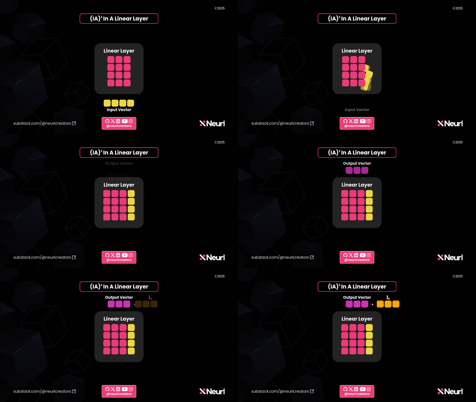
(IA)³ also introduces a third vector, but unlike the other two, it is not part of the attention mechanism. Instead, it is placed between the down projection and up projection layers.
Using (IA)³ in 🤗 PEFT
Just like we did with LoRA, we start by importing the configuration. In the configuration, we specify that we want to perform causal language modeling.
Then, we pass the model to the get_peft_model function, which creates a PEFT-enhanced model with (IA)³. Now, let’s take a look at the PEFT model.
Within the self_attn layer, you will notice that both k_proj and v_proj contain a module called ia3_l. This is a vector with dimensions 512 × 1, representing the (IA)³ vector we saw in the attention equation.
Similarly, within the down_proj layer, there is another ia3_l module. This corresponds to the third (IA)³ vector used in the feedforward layer.
(IA)³ Inference overhead and Downstream Performance
While (IA)³ is more efficient than LoRA during fine-tuning since it introduces vectors instead of weight matrices, unlike LoRA, which applies weight updates through simple addition, (IA)³ incorporates its updates as extra parameters. This increases the total number of parameters beyond the original model, leading to higher computational overhead during inference.
This inference overhead is common among most addition-based PEFT techniques. Moreover, while (IA)³ is more efficient during fine-tuning, that does not necessarily mean its downstream performance surpasses LoRA.
The paper Scaling Down to Scale Up: A Guide to Parameter-Efficient Fine-Tuning compared various PEFT techniques by fine-tuning T5 and its variants on natural language understanding (NLU) and natural language generation (NLG) tasks, including question answering and commonsense reasoning. The study evaluated (IA)³, LoRA (applied to just the Q and V matrices), LoRA (applied to all linear layers), and full fine-tuning.
Both LoRA methods outperformed all other techniques, and (IA)³ even fell short compared to full fine-tuning. This highlights that greater efficiency does not always translate to better performance in the world of PEFT.
Conclusion
Parameter-Efficient Fine-Tuning (PEFT) has made fine-tuning large language models more efficient and accessible to a wider audience, including companies, researchers, and hobbyists experimenting with LLMs. Libraries like 🤗 PEFT have further simplified the process with an intuitive API and well-structured documentation. Since it seamlessly integrates with other libraries in the Hugging Face ecosystem, it is a valuable addition to any AI builder’s toolkit.
This is just a glimpse of what the 🤗 PEFT library can do. Be sure to explore the official documentation to uncover more of its capabilities. Future deep dives will explore other aspects of the library and its integration with tools like TRL.


